For those of you unfamiliar with what a Gaussian polymer chain, I have to refer you to explanations in any reputable polymer science textbook. I'll eventually try to write an introduction myself, but I have to apologize, I just haven't had the time.
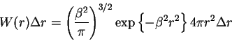
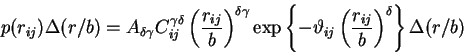
First I just explain where the Jacobson-Stockmayer (JS) equation comes from. We start with the familiar Gaussian polymer chain equation.
where
![]() ,
, ![]() is the monomer-to-monomer (or
mer-to-mer) separation distance between individual monomer on a
polymer chain and
is the monomer-to-monomer (or
mer-to-mer) separation distance between individual monomer on a
polymer chain and ![]() is the persistence length (a measure of the
correlation between individual monomers). The persistence length is
given in units of
is the persistence length (a measure of the
correlation between individual monomers). The persistence length is
given in units of ![]() (the mer-to-mer distance) and is usually greater
than
(the mer-to-mer distance) and is usually greater
than ![]() mer because. Some may note that
mer because. Some may note that
![]() if
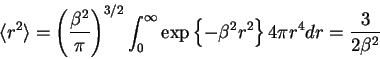
they have encountered other pages here. We then consider the
root-mean-square (RMS) end-to-end separation distance
if
they have encountered other pages here. We then consider the
root-mean-square (RMS) end-to-end separation distance
![]() in this expression
in this expression
where the RMS value itself is
![]() .
.
It is important to remember that the probability function
(1) is not expressing the length of the chain but the
end-to-end separation distance of monomer 1 and monomer ![]() (where an
RNA sequence is numbered as 1 at the 5' end and
(where an
RNA sequence is numbered as 1 at the 5' end and ![]() at the 3' end).
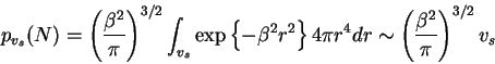
This RMS end-to-end separation distance has a finite
volume. Therefore, Jacobson and Stockmayer reasoned that the
probability that the two ends of the polymer chain of length
at the 3' end).
This RMS end-to-end separation distance has a finite
volume. Therefore, Jacobson and Stockmayer reasoned that the
probability that the two ends of the polymer chain of length ![]() will
localize within the same volume
will
localize within the same volume ![]() is
is
and because
![]() ,
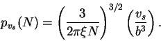
(3) simplifies to
,
(3) simplifies to
Given that one has chosen intelligent parameters for ![]() in relation
to
in relation
to ![]() , Eqn (4) is also a sensable probability
function to go further with. So, with no explicit temperature
dependence, the entropy is simply
, Eqn (4) is also a sensable probability
function to go further with. So, with no explicit temperature
dependence, the entropy is simply
![]() .
Therefore,
.
Therefore,
where ![]() is determined by estimates of
is determined by estimates of ![]() ,
,
![]() and
and ![]() . A similar expression was obtained by Poland and
Scheraga (1965) by a somewhat different and perhaps more
rigorous approach.
. A similar expression was obtained by Poland and
Scheraga (1965) by a somewhat different and perhaps more
rigorous approach.
In addition to this, some consideration was given to the fact that real polymers actually occupy space (a novel idea). The Gaussian polymer chain model is a random walk and does not care whether it crosses part of the path of a previous step. In fact, one possible structure is one in which you can fold the polymer back and forth between the same two points. This is obviously not physical. From the theoretical work of Fisher, it was shown that one effective solution is to change weight on the second term in Eqn (5) from 3/2 to about 1.75.
The key issue here is what values of ![]() would make sense. In these
models, one should perceive the supposed monomers in these models
(including ours) as some sort of spherical balls or a blobish sort of
collection of these balls whose individual center-of-mass corresponds
to the position of the drawn object. Most likely, one should not (for
typical blobs) expect that the center-of-mass of each blob would come
closer than the respective mer-to-mer separation distance (
would make sense. In these
models, one should perceive the supposed monomers in these models
(including ours) as some sort of spherical balls or a blobish sort of
collection of these balls whose individual center-of-mass corresponds
to the position of the drawn object. Most likely, one should not (for
typical blobs) expect that the center-of-mass of each blob would come
closer than the respective mer-to-mer separation distance (![]() ). In
short,
). In
short, ![]() . Indeed, a proper estimate for the distance
between the center-of-mass of each nucleic acid in a base-pair is
about
. Indeed, a proper estimate for the distance
between the center-of-mass of each nucleic acid in a base-pair is
about ![]() or
or
![]() . (One can see this is so by
considering the arrangement and general distances between the nucleic
acids in the base-pairs of a DNA helix and realize that it is at least
on the order of
. (One can see this is so by
considering the arrangement and general distances between the nucleic
acids in the base-pairs of a DNA helix and realize that it is at least
on the order of ![]() .) This renders
.) This renders ![]() far too small.
Therefore, the estimates from this parameter have usually been
empirical for RNA.
far too small.
Therefore, the estimates from this parameter have usually been
empirical for RNA.
What we call the ``JS-model'' is actually only such in the sense that we honor the variability of the weight (3/2) in Eqn (5). In fact, we show in our work that the JS-model is actually an approximation solution that satisfies a subset of our more general approach.
Here, we only say that the JS-model can be found by simplifying the McKenzie-Moore-Domb-Fisher distribution function. This model has the general form
where ![]() is the end-to-end separation distance between
two residues of index
is the end-to-end separation distance between
two residues of index ![]() and
and ![]() ,
, ![]() is a probability
distribution function used to express this end-to-end separation
distance,
is a probability
distribution function used to express this end-to-end separation
distance, ![]() is in part a factor in the self-avoiding (or
excluded volume) weight,
is in part a factor in the self-avoiding (or
excluded volume) weight, ![]() is the weight on the exponential
function,
is the weight on the exponential
function,
![]() is a dimensionless scaling parameter,
is a dimensionless scaling parameter,
![]() is the spherically symmetric solid angle weight
(not to be confused with
is the spherically symmetric solid angle weight
(not to be confused with ![]() in Eqn
(5)!!), and
in Eqn
(5)!!), and
![]() is a normalization
constant for the distribution function.
is a normalization
constant for the distribution function.
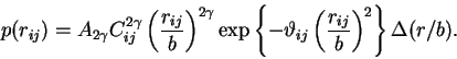
When
![]() , this equation becomes
, this equation becomes
Again, since there is no implicit temperature dependence, the entropy becomes the natural log of this expression,
In the JS equation, the change in entropy is measured from the
denatured structure (
![]() ) and the native state
(
) and the native state
(
![]() ), where
), where ![]() is a scalar constant
proportional to the separation between the two monomers when treated
as beads on a string and
is a scalar constant
proportional to the separation between the two monomers when treated
as beads on a string and ![]() is the root-mean-square separation
distance between
is the root-mean-square separation
distance between ![]() and
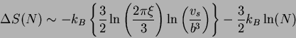
and ![]() in the denatured state. The resulting
loss in entropy as the structure folds from the denature state to the
native state has the form
in the denatured state. The resulting
loss in entropy as the structure folds from the denature state to the
native state has the form
where ![]() is the persistence length (a measure of the
correlation of the nucleotides at nearest neighboring ends),
is the persistence length (a measure of the
correlation of the nucleotides at nearest neighboring ends),
![]() is a constant with
is a constant with ![]() the base-pair separation
distance in units of
the base-pair separation
distance in units of ![]() . Since the free energy is
. Since the free energy is
![]() , for large
, for large ![]() , the leading contribution to the
free energy due to entropy loss has the form
, the leading contribution to the
free energy due to entropy loss has the form
![]() , which resembles the JS equation used in the Turner
energy rules.
, which resembles the JS equation used in the Turner
energy rules.
It is for this reason that we honor the tradition of calling this the JS-model. However, it should be firmly planted in the reader's mind that this bears but a superficial resemblance to the JS-model traditionally used in the dynamic programming algorithm and only reduced to such under limiting conditions.