The origin of this model is largely the pioneering work of these
individuals. Fisher was the first to recognize and find a
parameterization for the non-Gaussian character of the distribution
function. The constant ![]() in the Gaussian-like function
used in Mfold and the Vienna package has its origins in Fisher's work.
Domb and Fisher both did a fair amount of study on the exponent, and
McKenzie and Moore established further justification for working on the
weight for the self-avoiding walk.
in the Gaussian-like function
used in Mfold and the Vienna package has its origins in Fisher's work.
Domb and Fisher both did a fair amount of study on the exponent, and
McKenzie and Moore established further justification for working on the
weight for the self-avoiding walk.
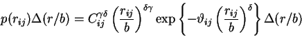
In the most general expression for the distribution function, the
likelihood of finding mers ![]() and
and ![]() with an end-to-end separation
distance of
with an end-to-end separation
distance of ![]() and contained within a volume element of
and contained within a volume element of
![]() is
is
where ![]() is a weight that accounts for the
self-avoiding character of the polymer and contributes to the the
excluded volume,
is a weight that accounts for the
self-avoiding character of the polymer and contributes to the the
excluded volume, ![]() is the weight on the exponential function,
and
is the weight on the exponential function,
and
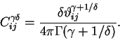
![]() is a normalization constant for the
distribution function
is a normalization constant for the
distribution function
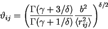
where ![]() is a Gamma-function. The constant
is a Gamma-function. The constant
![]() is is a dimensionless scaling parameter that is a
function of the root-mean-square (rms) end-to-end separation-distance
of the polymer chain,
is is a dimensionless scaling parameter that is a
function of the root-mean-square (rms) end-to-end separation-distance
of the polymer chain,
In its most general form,
where ![]() is an unspecified weight factor,
is an unspecified weight factor, ![]() is
the persistence length (a measure of the correlation) and
is
the persistence length (a measure of the correlation) and ![]() is the
weight on
is the
weight on ![]() . It seems best to say that one should generally assume
that
. It seems best to say that one should generally assume
that
![]() in these problems without serious evidence
to the contrary. The central limit theorem predicts that
in these problems without serious evidence
to the contrary. The central limit theorem predicts that
![]() for a GPC; however, some aspects of RNA behavior tend to deviate
from this ideal situation. The persistence length is a
measure of the correlation between segments in a polymer.
for a GPC; however, some aspects of RNA behavior tend to deviate
from this ideal situation. The persistence length is a
measure of the correlation between segments in a polymer.
This function assumes that the characteristics of the polymer can be
reduced to nearly identical entities to a reasonable approximation.
For the most part, the four bases in RNA can broadly meet these
attributes. When
![]() and
and
![]() ,
, ![]() becomes a Gaussian function that is the origin of its name Gaussian
polymer chain (GPC).
becomes a Gaussian function that is the origin of its name Gaussian
polymer chain (GPC).
A central theme in approaches that use this kind of model is
![]() resembles a Gaussian polymer chain (GPC). When
resembles a Gaussian polymer chain (GPC). When ![]() is Gaussian, the parameters in (1) become
is Gaussian, the parameters in (1) become
![]() and
and
![]() . The strict model of the GPC
maintains
. The strict model of the GPC
maintains
![]() ; however, since a Gaussian function is a
special case of a more general family known as
; however, since a Gaussian function is a
special case of a more general family known as ![]() -functions,
altering this parameter in (1) has for the most part
the effect of changing the weight on equation but otherwise not
affecting the general properties. Without invoking the ``-flory''
option, it is assume that
-functions,
altering this parameter in (1) has for the most part
the effect of changing the weight on equation but otherwise not
affecting the general properties. Without invoking the ``-flory''
option, it is assume that ![]() .
.
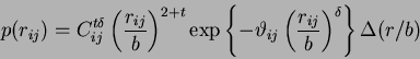
In the McKenzie-Domb (McD) equations, eq (1) is altered slightly to the form
hence,
![]() .
.
The model strongly built around a continuum renormalization theory to get the correct polymer distribution function. Because of the difficulty of such models, they generally are restricted to the polymer in good solvent where strong self-(attractive)-interactions can be sufficiently ignored. Exactly what happens when you allow for strong self-interactions is a lot murkier. This model is provided as is. There are many problems with continuum renormalization theory that are difficult to address particularly when self-interaction is strong. The strong point of the continuum renormalization method is that reveals critical constants.