


Next: Flory terms and the
Up: A generalized solvent-polymer interaction
Previous: Van der Waals equation
A model for polymers
Having now worked through the Van der Waals mean field approach and having
introduced the approach used in Flory's model with the entropy of mixing, we
now seek to place the polymer-solvent equations into perspective.
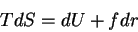
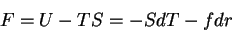
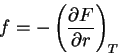
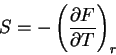
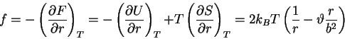
First, the thermodynamic potentials should be modified to reflect the state
variables used in polymers. We seek  and
and  . The equations of
state become
. The equations of
state become
 |
(65) |
 |
(66) |
 |
(67) |
 |
(68) |
 |
(69) |
 |
(70) |
We start by considering the GPC solution as originally found in Flory's
model (
 and
and
 . In the case of an ideal
polymer, the equation of state is found by using the analogous equation for
. In the case of an ideal
polymer, the equation of state is found by using the analogous equation for
 :
:  ,
,
 . For the GPC,
 |
(71) |
and
 |
(72) |
because
 just as
 for the ideal gas. Equation (72) represents an equation of
state for a polymer analogous to
for the ideal gas. Equation (72) represents an equation of
state for a polymer analogous to 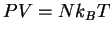 for the ideal gas.
Now, if there are additional terms such as the excluded volume, we must
introduce two-body and three-body density dependent term into an expression
for the free energy as a function of swelling. The internal interaction of
the chain are expressed as in the Flory case as
 (39)
(39)
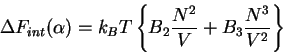 |
(73) |
where  corresponds to (59) and
  corresponds to (60). Now we make
the approximation that
corresponds to (60). Now we make
the approximation that
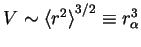 . This is justified because the rms end-to-end separation
distance is a function of the actual volume of the polymer. Using the fact
that
. This is justified because the rms end-to-end separation
distance is a function of the actual volume of the polymer. Using the fact
that
 , we obtain
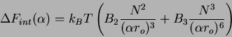 |
(74) |
For the elastic contribution (
 , we again call
forth (13). As previously in (44), the total FE from this process is the sum
of
and
, we again call
forth (13). As previously in (44), the total FE from this process is the sum
of
and
 |
(75) |
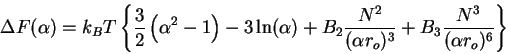
Then taking the derivative
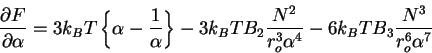 |
(76) |
and solving for the stationary points, we obtain the famous Flory expression
again with additional information on the relationship for and ,
 |
(77) |
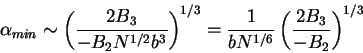
where in good solvent, one can typically ignore the constant contribution of
. The relationship between and can, in principle, be
found either by calculation or by experiment. In the limiting case of large
 and in good solvent conditions, one can see that the dominant term is
and
and in good solvent conditions, one can see that the dominant term is
and  as a function of must be
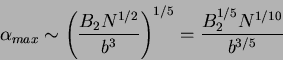 |
(78) |
where  .
.
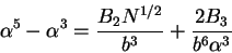
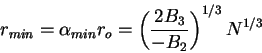
For a polymer in poor solvent, one finds a situation where is
negative and both and are significant. In such cases, we
should rewrite (77) as
 |
(79) |
In the limiting case of large , (79) reduces to
 |
(80) |
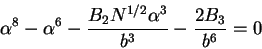
Solving for  we in (77) and (79) obtain
 |
(81) |
and
 |
(82) |
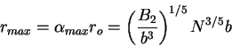
where has units of volume and volume squared.
Hence, we obtain Flory's original
 dependence and the
corresponding globular case where
dependence and the
corresponding globular case where
 .
.
Finally, for completeness, we write the general form for (77) which can be
found by substituting (13) into (75) and following the same procedures,
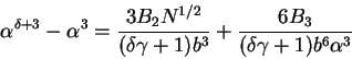 |
(83) |
One can quickly see that for
and
 , (83)
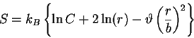
reduces to (77). Moreover, applying the renormalization group solution of
, (83)
reduces to (77). Moreover, applying the renormalization group solution of
 into (83), one obtains
 ;
almost precisely the renormalization group estimated value for
;
almost precisely the renormalization group estimated value for  .
Renormalization group theory has not been discussed at all here and is only
briefly described in the McKenzie-Moore-Domb-Fisher model, but little need
be said about the importance of establishing a sense of unity between
different strategies. Indeed, the independent approach of the Flory model
appears to have generated some values of the critical exponent that are
surprisingly consistent with renormalization group theory.
.
Renormalization group theory has not been discussed at all here and is only
briefly described in the McKenzie-Moore-Domb-Fisher model, but little need
be said about the importance of establishing a sense of unity between
different strategies. Indeed, the independent approach of the Flory model
appears to have generated some values of the critical exponent that are
surprisingly consistent with renormalization group theory.
Next: Flory terms and the
Up: A generalized solvent-polymer interaction
Previous: Van der Waals equation
Wayne Dawson
2007-01-10