In the previous sections, we have essentially ignored the dependence of the
persistence length on the expressions for polymer-solvent interaction. The
program does not assume that the structure of the polymer is at the
convenience of our eyes and or reagents. Rather, the program is concerned
with how nature has reduced the number of degrees of freedom on the
biopolymer to produce the structure one sees in the journal or the textbook.
Having a persistence length different from ![]() means that we must
divide the sequence into
means that we must
divide the sequence into ![]() ``effective'' mers each of which has a
length
``effective'' mers each of which has a
length ![]() . The total length of the stretched out sequence is therefore
the same:
. The total length of the stretched out sequence is therefore
the same:
![]() , but the manipulation does require some
modification.
, but the manipulation does require some
modification.
Three parameters are needed to describe ![]() :
: ![]() ,
, ![]() and
and ![]() .
Using the definition
.
Using the definition
![]() as the unperturbed rms end-to-end
separation-distance, we write
as the unperturbed rms end-to-end
separation-distance, we write ![]() as
as
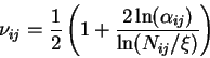
To handle the general case of stacking in RNA, one must estimate the rms
end-to-end separation-distance for each base-pair ![]() in the polymer
chain rather than just the extreme ends (
in the polymer
chain rather than just the extreme ends (![]() and
and ![]() .
Therefore, the model must be modified slightly because the
.
Therefore, the model must be modified slightly because the ![]() parameter depends on the length of the chain, yet all chain lengths of the
same polymer must exhibit the same
parameter depends on the length of the chain, yet all chain lengths of the
same polymer must exhibit the same ![]() dependence on
dependence on ![]() . Since each order pair
. Since each order pair
![]() must exhibit this same property, one single
must exhibit this same property, one single ![]() parameter is
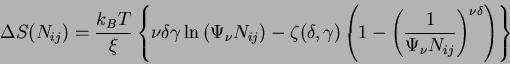
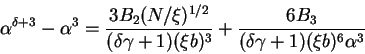
simply not appropriate. Then the result for
parameter is
simply not appropriate. Then the result for ![]() follows from
(86)
follows from
(86)
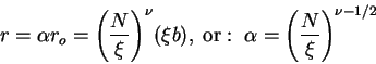
The limits on ![]() and the corresponding polymer-solvent conditions and
the corresponding virial coefficients are summarized in Table 1.
and the corresponding polymer-solvent conditions and
the corresponding virial coefficients are summarized in Table 1.
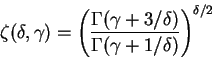
The exponent ![]() can be expressed as a function of
can be expressed as a function of ![]() through the following relationship
through the following relationship
|