In the thermodynamics of gas models, people have often turned to lattice
models to solve many statistical mechanics problems. At first sight, a
lattice may seem strange because a gas is hardly stable like a crystal of
quartz. However, if we were to take many instantaneous snap shots of a gas
in motion, and average what we see, we would begin to see a very blurry
picture that somewhat resembled a lattice because of the mutual repulsion of
the gas both to itself and to the walls of the container. Similarly, liquids
are even closer to crystals. Glass does not have long range order like a
regular crystal lattice, but the local coordination of the various SiO![]() molecules is hardly random in character. Aside from more extensive defects,
the local coordination resembles quartz in many ways. Statistical mechanics
is about the long time range characteristics of a system, not the
instantaneous activity. Thus, a lattice model should not be seen as all that
strange or unphysical.
molecules is hardly random in character. Aside from more extensive defects,
the local coordination resembles quartz in many ways. Statistical mechanics
is about the long time range characteristics of a system, not the
instantaneous activity. Thus, a lattice model should not be seen as all that
strange or unphysical.
Flory's theory was derived from these often used lattice-models where he considered the entropy of mixing of a polymer solvent system where the concentration of solvent was small relative to the polymer. The entropy of mixing measures the change in free volume due to replacement of one type of molecule by another.
Let index ![]() refers to the solvent and index
refers to the solvent and index ![]() refers to the polymer. The
volume occupied by a polymer is much larger than the volume occupied by a
typical solvent; usually by a very large factor. Flory reasoned that one
must account for this by considering the number of segments
refers to the polymer. The
volume occupied by a polymer is much larger than the volume occupied by a
typical solvent; usually by a very large factor. Flory reasoned that one
must account for this by considering the number of segments ![]() in the
polymer; not just the mole fraction of polymer or solvent. He noted that the
volume of the polymer-segments may also be different from that of the
solvent, but in first approximation, these are mere corrections and a
lattice model could account for that in principle. For a binary system of
solvent and polymer with mole fraction of solvent (
in the
polymer; not just the mole fraction of polymer or solvent. He noted that the
volume of the polymer-segments may also be different from that of the
solvent, but in first approximation, these are mere corrections and a
lattice model could account for that in principle. For a binary system of
solvent and polymer with mole fraction of solvent (![]() and polymer (
and polymer (![]() , the total volume of the polymer and solvent should be
, the total volume of the polymer and solvent should be ![]() . The
corresponding volume fraction of solvent is
. The
corresponding volume fraction of solvent is
![]() and
polymer
and
polymer
![]() . Hence,
. Hence,
![]() .
.
By considering the volume fraction as opposed to the mole fraction, the
accuracy of the entropy of mixing (Raoult's law) is greatly improved
Now, the enthalpy of solvation is obtained from the van Laar expression for
the heat of mixing in a two component system (here solvent and polymer)
In Flory's model,
From (15) and (17), the free energy (FE) of mixing
(![]() can now be written down as
can now be written down as
and the chemical potential of the solvent comes from differentiating
(19) with respect to ![]() (and noting that
(and noting that ![]() and
and ![]() are functions of
are functions of ![]() and
and ![]() yields
yields
where ![]() is the number of segments.
is the number of segments.
This expression is only valid for dilute solvent but the main
point of interest is for dilute polymer solutions. This was
the issue raised in invoking Raoult's law in the first place. Why is
this important? Equation (20) follows directly from
(19) when the partial derivative is used with ![]() constant
and then setting
constant
and then setting ![]() . However, because the definition of
. However, because the definition of
![]() (
(![]() is known, it is better to use the total
derivative. Doing so, equation (20) results only when the
assumed conditions are the following:
is known, it is better to use the total
derivative. Doing so, equation (20) results only when the
assumed conditions are the following: ![]() ,
, ![]() and
and ![]() . In short, (20) is valid when
. In short, (20) is valid when ![]() . The
solution for the first term should actually contain
. The
solution for the first term should actually contain ![]() and
there are other surviving terms in
and
there are other surviving terms in ![]() and
and ![]() when the total
derivative is used.
when the total
derivative is used.
This problem emerges in part because of the way this expression is derived.
From the stand point of the excluded volume for a gas, we have

The argument is now shifted to volume elements from the viewpoint that in dilute polymer solutions, the polymer-solvent system will consist of isolated molecules of the polymer surrounded by a large open regions occupied by the solvent. Within a small volume element at the location of the given polymer, the environment will resemble the dilute solvent condition where (20) is still valid (in principle)
where ![]() emphasizes that we are working with a
volume element and not the bulk system.
emphasizes that we are working with a
volume element and not the bulk system.
It is convenient to expand ![]() in a power series
in a power series
One serious objection here is that the presumed conditions
are those of a polymer rich solution yet we have invoked a power
series approximation of ![]() as though it were small and guaranteed
convergence. This is not a minor point either because the logarithmic
term essentially explodes when
as though it were small and guaranteed
convergence. This is not a minor point either because the logarithmic
term essentially explodes when ![]() .
.
Nevertheless, proceeding, we simplify (22) to obtain the following
where
![]() and
and
![]() with
with ![]() and
and ![]() the enthalpy
and entropy of mixing the solvent with the given polymer.
the enthalpy
and entropy of mixing the solvent with the given polymer.
From this formulation, we define a parameter ![]()
where the ![]() -temperature represents the ideal
temperature at which Van't Hoff's law is obeyed for a given
solvent-polymer system. Substituting into (23), we have
-temperature represents the ideal
temperature at which Van't Hoff's law is obeyed for a given
solvent-polymer system. Substituting into (23), we have
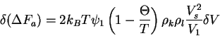
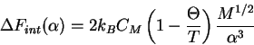
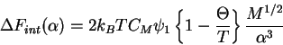
The excess chemical potential is then
This provides the basis for the equation for the ![]() point.
point.
Now that we have shown how to arrive at an expression for the ![]() point, we return to (19) to find a way to express the excluded
volume of two segments or parts of the same polymer segment. The
reason for having side tracked a bit is because the
point, we return to (19) to find a way to express the excluded
volume of two segments or parts of the same polymer segment. The
reason for having side tracked a bit is because the ![]() point is
so central to Flory's theory and it appears in many places. Without
showing where this (25) comes from, it is rather hard to
explain how it drops into the other things we need to look at later.
point is
so central to Flory's theory and it appears in many places. Without
showing where this (25) comes from, it is rather hard to
explain how it drops into the other things we need to look at later.
We consider two volume elements ![]() and
and ![]() . We
introduce the concept of ``segment densities'' for the polymer
segments
. We
introduce the concept of ``segment densities'' for the polymer
segments ![]() and
and ![]() :
: ![]() and
and ![]() respectively (units:
number of segments per unit volume). Let
respectively (units:
number of segments per unit volume). Let ![]() be the volume of such
a segment. (I know, haven't we endured enough parameters yet?.... It
seems relevant to me because it is hard to grasp the usage of these
parameterizations without showing where they come from. Once we
understand that point, then it is easier to see the connection between
Flory's work and concepts a little more familiar to us.).
be the volume of such
a segment. (I know, haven't we endured enough parameters yet?.... It
seems relevant to me because it is hard to grasp the usage of these
parameterizations without showing where they come from. Once we
understand that point, then it is easier to see the connection between
Flory's work and concepts a little more familiar to us.).
The volume fraction in each of the polymer elements is
where the index ![]() refers to the ``polymer''. If the two
volume elements are brought to a separation distance
refers to the ``polymer''. If the two
volume elements are brought to a separation distance ![]() , the combined
concentration will be simply
, the combined
concentration will be simply
If we now consider that the volume is mostly occupied by
solvent in the regions between these two polymer segments, then we can
approximate the total volume by the volume of the solvent ![]() (
(![]() , where
, where ![]() is Avogadro's number). The number of
solvent molecules in
is Avogadro's number). The number of
solvent molecules in ![]() (the region containing both
(the region containing both ![]() and
and
![]() , will be
, will be
hence,
Rewriting (19) for
![]() for example, we obtain
for example, we obtain
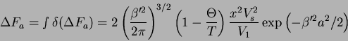
and making all the necessary substitutions with equations (27-30), the change in the activity is
and with a little algebra, one arrives at
where the product
![]() is where we eventually
will arrive at the
is where we eventually
will arrive at the ![]() dependence in the excluded volume term.
dependence in the excluded volume term.
To fight our way through this last matter, we need to define ![]() and
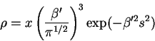
and ![]() . Flory assumes a radial dependence on the segment
density
. Flory assumes a radial dependence on the segment
density
where ![]() is defined as before as the total number of
segments in the molecule. According to the general theory for the
radius of gyration
is defined as before as the total number of
segments in the molecule. According to the general theory for the
radius of gyration
![]() and
and
![]() . For a Gaussian distribution function as (34),
we have
. For a Gaussian distribution function as (34),
we have
where we find the relationship between ![]() and
and ![]() is
is
![]() or
or
![]() .
.
Now we land on some shaky material again. I don't really find the
method works so well here, but what we want to do is evaluate
![]() in a similar way as
(35). I think the strategy used by Flory here to get the joint
distribution function is a bit questionable, but I will explain what
was done. First, you assume cylindrical symmetry and claim that
in a similar way as
(35). I think the strategy used by Flory here to get the joint
distribution function is a bit questionable, but I will explain what
was done. First, you assume cylindrical symmetry and claim that ![]() and
and ![]() can be expressed as follows
can be expressed as follows
so finally we have
Now!, with just a few more definitions, we are
about through the difficult part of this discussion.... Let the volume
of a segment ![]() be related to the number of segments
be related to the number of segments ![]() as
follows:
as
follows:
![]() where
where ![]() is the molar
specific volume of polymer and
is the molar
specific volume of polymer and ![]() is its molecular weight. Further,
let
is its molecular weight. Further,
let ![]() as indicated earlier, where
as indicated earlier, where ![]() is Avogadro's
number and
is Avogadro's
number and ![]() is the volume fraction of solvent (
is the volume fraction of solvent (
![]() .
.
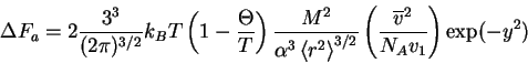
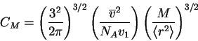
After doing some more substitution, we arrive at
Now that we have gathered together this large throng of symbols, we are now in the position to develop Flory's famous formula. Parameters associated with the Mayer function and the excluded volume can also be obtained using this approach. The derivations are tedious and major objections can be raised at several steps. Despite these flaws, the interested reader is encouraged to consult the literature to learn how these steps are done for their own edification.
The free energy consists of both an elastic contribution due to the polymer swelling (or contracting), and an internal interaction caused by the interaction of the polymer with itself and with the solvent surrounding it
where, for a GPC,
and likewise
Then, combining (42) and (43) together in
(41), the total FE for swelling (or contracting) for the
polymer chain of length ![]() as measured at the rms end-to-end
separation distance is
as measured at the rms end-to-end
separation distance is
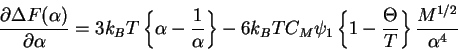
Finally, we now try to minimize this expression
and, taking the stationary point, we obtain
Considering that
![]() , (46) simplifies to
, (46) simplifies to
which is Flory's famous solvent swelling expression.
Although we have presented a rough introduction to the original means by
which Flory found this property of polymers, in fact, this large cavalcade
of parameters does not help bring about significant agreement with
experiment for most systems. The important prediction from this theory is
the ![]() dependence for polymers in good solvent that we will show
later.
dependence for polymers in good solvent that we will show
later.